Introduction to package `nngeo`

Introduction

Package purpose

This document introduces the nngeo package. The nngeo package includes functions for spatial join of layers based on k-nearest neighbor relation between features. The functions work with spatial layer object defined in package sf, namely classes sfc and sf.

Installation

CRAN version:

install.packages("remotes")
remotes::install_github("michaeldorman/nngeo")

GitHub version:

install.packages("nngeo")

Sample data

The nngeo package comes with three sample datasets:

cities
towns
water

The cities layer is a point layer representing the location of the three largest cities in Israel.

cities
#> Simple feature collection with 3 features and 1 field
#> Geometry type: POINT
#> Dimension:     XY
#> Bounding box:  xmin: 34.78177 ymin: 31.76832 xmax: 35.21371 ymax: 32.79405
#> Geodetic CRS:  WGS 84
#>        name                  geometry
#> 1 Jerusalem POINT (35.21371 31.76832)
#> 2  Tel-Aviv  POINT (34.78177 32.0853)
#> 3     Haifa POINT (34.98957 32.79405)

The towns layer is another point layer, with the location of all large towns in Israel, compiled from a different data source:

towns
#> Simple feature collection with 193 features and 4 fields
#> Geometry type: POINT
#> Dimension:     XY
#> Bounding box:  xmin: 34.27 ymin: 29.56 xmax: 35.6 ymax: 33.21
#> Geodetic CRS:  WGS 84
#> First 10 features:
#>             name country.etc   pop capital            geometry
#> 12        'Afula      Israel 39151       0 POINT (35.29 32.62)
#> 17         'Akko      Israel 45606       0 POINT (35.08 32.94)
#> 40       'Ar'ara      Israel 15841       0  POINT (35.1 32.49)
#> 41         'Arad      Israel 22757       0 POINT (35.22 31.26)
#> 43       'Arrabe      Israel 20316       0 POINT (35.33 32.85)
#> 52        'Atlit      Israel  4686       0 POINT (34.93 32.68)
#> 103     'Eilabun      Israel  4296       0  POINT (35.4 32.83)
#> 104   'Ein Mahel      Israel 11014       0 POINT (35.35 32.72)
#> 105 'Ein Qiniyye      Israel  2101       0 POINT (35.15 31.93)
#> 112        'Ilut      Israel  6536       0 POINT (35.25 32.72)

The water layer is an example of a polygonal layer. This layer contains four polygons of water bodies in Israel.

water
#> Simple feature collection with 4 features and 1 field
#> Geometry type: POLYGON
#> Dimension:     XY
#> Bounding box:  xmin: 34.1388 ymin: 29.45338 xmax: 35.64979 ymax: 33.1164
#> Geodetic CRS:  WGS 84
#>                name                       geometry
#> 1           Red Sea POLYGON ((34.96428 29.54775...
#> 2 Mediterranean Sea POLYGON ((35.10533 33.07661...
#> 3          Dead Sea POLYGON ((35.54743 31.37881...
#> 4    Sea of Galilee POLYGON ((35.6014 32.89248,...

Figure $\ref{fig:layers}$ shows the spatial configuration of the cities, towns and water layers.

plot(st_geometry(water), col = "lightblue")
plot(st_geometry(towns), col = "grey", pch = 1, add = TRUE)
plot(st_geometry(cities), col = "red", pch = 1, add = TRUE)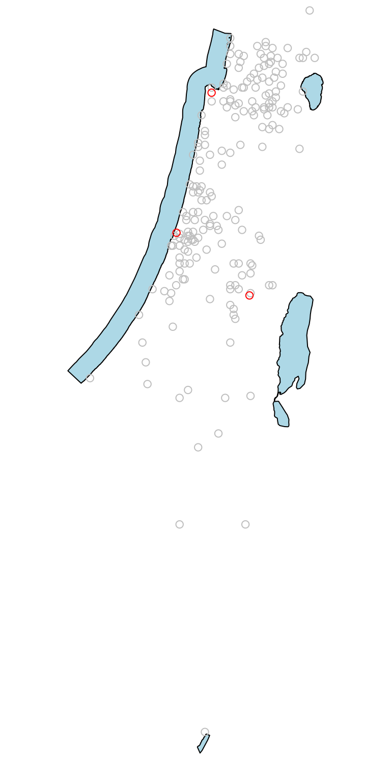

$Visualization of the \texttt{water}, \texttt{towns} and \texttt{cities} layers$

Visualization of the , and layers

Usage examples

The `st_nn` function

The main function in the nngeo package is st_nn. The st_nn function accepts two layers, x and y, and returns a list with the same number of elements as x features. Each list element i is an integer vector with all indices j for which x[i] and y[j] are nearest neighbors.

For example, the following expression finds which feature in towns is the nearest neighbor to each feature in cities:

nn = st_nn(cities, towns, progress = FALSE)
#> lon-lat points
nn
#> [[1]]
#> [1] 70
#> 
#> [[2]]
#> [1] 145
#> 
#> [[3]]
#> [1] 59

This output tells us that towns[70, ] is the nearest among the 193 features of towns to cities[1, ], towns[145, ] is the nearest to cities[2, ], and towns[59, ] is the nearest to cities[3, ].

The `st_connect` function

The resulting nearest neighbor matches can be visualized using the st_connect function. This function builds a line layer connecting features from two layers x and y based on the relations defined in a list such the one returned by st_nn:

l = st_connect(cities, towns, ids = nn)
#> Calculating nearest IDs
#> Calculating lines
l
#> Geometry set for 3 features 
#> Geometry type: LINESTRING
#> Dimension:     XY
#> Bounding box:  xmin: 34.78177 ymin: 31.76832 xmax: 35.22 ymax: 32.82
#> Geodetic CRS:  WGS 84
#> LINESTRING (35.21371 31.76832, 35.22 31.78)
#> LINESTRING (34.78177 32.0853, 34.8 32.08)
#> LINESTRING (34.98957 32.79405, 34.99 32.82)

Plotting the line layer l gives a visual demonstration of the nearest neighbors match, as shown in Figure $\ref{fig:st_connect}$.

plot(st_geometry(l))
plot(st_geometry(towns), col = "darkgrey", add = TRUE)
plot(st_geometry(cities), col = "red", add = TRUE)
text(st_coordinates(cities)[, 1], st_coordinates(cities)[, 2], 1:3, col = "red", pos = 4)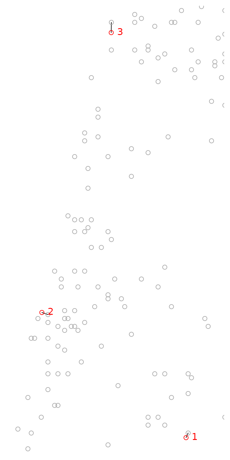

$Nearest neighbor match between \texttt{cities} (in red) and \texttt{towns} (in grey)$

Nearest neighbor match between (in red) and (in grey)

Dense matrix representation

The st_nn can also return the complete logical matrix indicating whether each feature in x is a neighbor of y. To get the dense matrix, instead of a list, use sparse=FALSE.

nn = st_nn(cities, towns[1:5, ], sparse = FALSE, progress = FALSE)
#> lon-lat points
nn
#>       [,1]  [,2]  [,3]  [,4]  [,5]
#> [1,] FALSE FALSE FALSE  TRUE FALSE
#> [2,] FALSE FALSE  TRUE FALSE FALSE
#> [3,] FALSE  TRUE FALSE FALSE FALSE

k-Nearest neighbors where `k>0`

It is also possible to return any k-nearest neighbors, rather than just one. For example, setting k=2 returns both the 1^st and 2^nd nearest neighbors:

nn = st_nn(cities, towns, k = 2, progress = FALSE)
#> lon-lat points
nn
#> [[1]]
#> [1] 70 99
#> 
#> [[2]]
#> [1] 145 175
#> 
#> [[3]]
#> [1]  59 179

Here is another example, finding the 10-nearest neighbor towns features for each cities feature:

x = st_nn(cities, towns, k = 10)
#> lon-lat points
l = st_connect(cities, towns, ids = x)

The result is visualized in Figure $\ref{fig:cities_towns}$.

plot(st_geometry(l))
plot(st_geometry(cities), col = "red", add = TRUE)
plot(st_geometry(towns), col = "darkgrey", add = TRUE)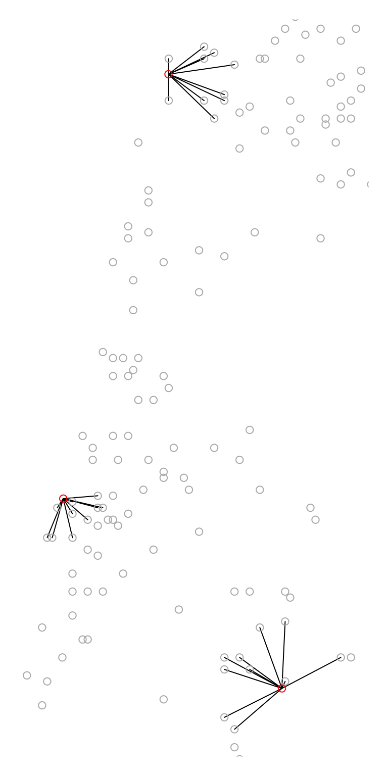

$Nearest 10 \texttt{towns} features from each \texttt{cities} feature$

Nearest 10 features from each feature

Distance to nearest neighbors

Using returnDist=TRUE the distances list is also returned, in addition the the neighbor matches, with both components now comprising a list:

nn = st_nn(cities, towns, k = 1, returnDist = TRUE, progress = FALSE)
#> lon-lat points
nn
#> $nn
#> $nn[[1]]
#> [1] 70
#> 
#> $nn[[2]]
#> [1] 145
#> 
#> $nn[[3]]
#> [1] 59
#> 
#> 
#> $dist
#> $dist[[1]]
#> [1] 1425.692
#> 
#> $dist[[2]]
#> [1] 1818.853
#> 
#> $dist[[3]]
#> [1] 2878.572

Search radius

Finally, the search for nearest neighbors can be limited to a search radius using maxdist. In the following example, the search radius is set to 2,000 meters (2 kilometers). Note that no neighbors are found within the search radius for cities[3, ], therefore the third list element is a zero-length vector of indices:

nn = st_nn(cities, towns, k = 1, maxdist = 2000, progress = FALSE)
#> lon-lat points
nn
#> [[1]]
#> [1] 70
#> 
#> [[2]]
#> [1] 145
#> 
#> [[3]]
#> integer(0)

Spatial join

The st_nn function can also be used as a predicate function when performing spatial join with sf::st_join. For example, the following expression spatially joins the two nearest towns features to each cities features, using a search radius of 5 km:

st_join(cities, towns, join = st_nn, k = 2, maxdist = 5000, progress = FALSE)
#> lon-lat points
#> Simple feature collection with 5 features and 5 fields
#> Geometry type: POINT
#> Dimension:     XY
#> Bounding box:  xmin: 34.78177 ymin: 31.76832 xmax: 35.21371 ymax: 32.79405
#> Geodetic CRS:  WGS 84
#>        name.x        name.y country.etc    pop capital
#> 1   Jerusalem     Jerusalem      Israel 731731       1
#> 2    Tel-Aviv     Ramat Gan      Israel 128583       0
#> 2.1  Tel-Aviv Tel Aviv-Yafo      Israel 384276       0
#> 3       Haifa         Haifa      Israel 266418       0
#> 3.1     Haifa  Tirat Karmel      Israel  19080       0
#>                      geometry
#> 1   POINT (35.21371 31.76832)
#> 2    POINT (34.78177 32.0853)
#> 2.1  POINT (34.78177 32.0853)
#> 3   POINT (34.98957 32.79405)
#> 3.1 POINT (34.98957 32.79405)

Binding distances to join result

Sometimes it’s necessary to bind the distances to the joined features in the resulting layer, to have more detailed information about the distance to nearest features. For example, suppose we join the nearest towns feature to cities, as shown above:

cities1 = st_join(cities, towns, join = st_nn, k = 1, progress = FALSE)
#> lon-lat points
cities1
#> Simple feature collection with 3 features and 5 fields
#> Geometry type: POINT
#> Dimension:     XY
#> Bounding box:  xmin: 34.78177 ymin: 31.76832 xmax: 35.21371 ymax: 32.79405
#> Geodetic CRS:  WGS 84
#>      name.x    name.y country.etc    pop capital                  geometry
#> 1 Jerusalem Jerusalem      Israel 731731       1 POINT (35.21371 31.76832)
#> 2  Tel-Aviv Ramat Gan      Israel 128583       0  POINT (34.78177 32.0853)
#> 3     Haifa     Haifa      Israel 266418       0 POINT (34.98957 32.79405)

As shown above, the distances can be calculated using the returnDist=TRUE option, then binded to the above join result:

# Calculate distances
n = st_nn(cities, towns, k = 1, returnDist = TRUE, progress = FALSE)
#> lon-lat points
dists = sapply(n[[2]], "[", 1)
dists
#> [1] 1425.692 1818.853 2878.572

# Bind distances
cities1$dist = dists
cities1
#> Simple feature collection with 3 features and 6 fields
#> Geometry type: POINT
#> Dimension:     XY
#> Bounding box:  xmin: 34.78177 ymin: 31.76832 xmax: 35.21371 ymax: 32.79405
#> Geodetic CRS:  WGS 84
#>      name.x    name.y country.etc    pop capital                  geometry
#> 1 Jerusalem Jerusalem      Israel 731731       1 POINT (35.21371 31.76832)
#> 2  Tel-Aviv Ramat Gan      Israel 128583       0  POINT (34.78177 32.0853)
#> 3     Haifa     Haifa      Israel 266418       0 POINT (34.98957 32.79405)
#>       dist
#> 1 1425.692
#> 2 1818.853
#> 3 2878.572

In the above workflow, we actually ran the same nearest neighbor search twice, once in st_join and more time to get the distances.

Another more verbose approach can be used in case the computation time is prohibitive. Here, we calculate the nearest neighbor indices and distances just once, then use them to construct the “joined” table with the distances:

# Get indices & distances
n = st_nn(cities, towns, k = 1, returnDist = TRUE, progress = FALSE)
#> lon-lat points
ids = sapply(n[[1]], "[", 1)
dists = sapply(n[[2]], "[", 1)

# Join
cities1 = data.frame(cities, st_drop_geometry(towns)[ids, , drop = FALSE])
cities1 = st_sf(cities1)

# Add distances
cities1$dist = dists
cities1
#> Simple feature collection with 3 features and 6 fields
#> Geometry type: POINT
#> Dimension:     XY
#> Bounding box:  xmin: 34.78177 ymin: 31.76832 xmax: 35.21371 ymax: 32.79405
#> Geodetic CRS:  WGS 84
#>        name    name.1 country.etc    pop capital                  geometry
#> 1 Jerusalem Jerusalem      Israel 731731       1 POINT (35.21371 31.76832)
#> 2  Tel-Aviv Ramat Gan      Israel 128583       0  POINT (34.78177 32.0853)
#> 3     Haifa     Haifa      Israel 266418       0 POINT (34.98957 32.79405)
#>       dist
#> 1 1425.692
#> 2 1818.853
#> 3 2878.572

Polygons

Nearest neighbor search also works for non-point layers. The following code section finds the 20-nearest towns features for each water body in water[-1, ].

nn = st_nn(water[-1, ], towns, k = 20, progress = FALSE)
#> lines or polygons

Again, we can calculate the respective lines for the above result using st_connect. Since one of the inputs is line/polygon, we need to specify a sampling distance dist, which sets the resolution of connecting points on the shape exterior boundary.

l = st_connect(water[-1, ], towns, ids = nn, dist = 100)
#> Calculating nearest IDs
#> Calculating lines

The result is visualized in Figure $\ref{fig:water_towns}$.

plot(st_geometry(water[-1, ]), col = "lightblue", border = "grey")
plot(st_geometry(towns), col = "darkgrey", add = TRUE)
plot(st_geometry(l), col = "red", add = TRUE)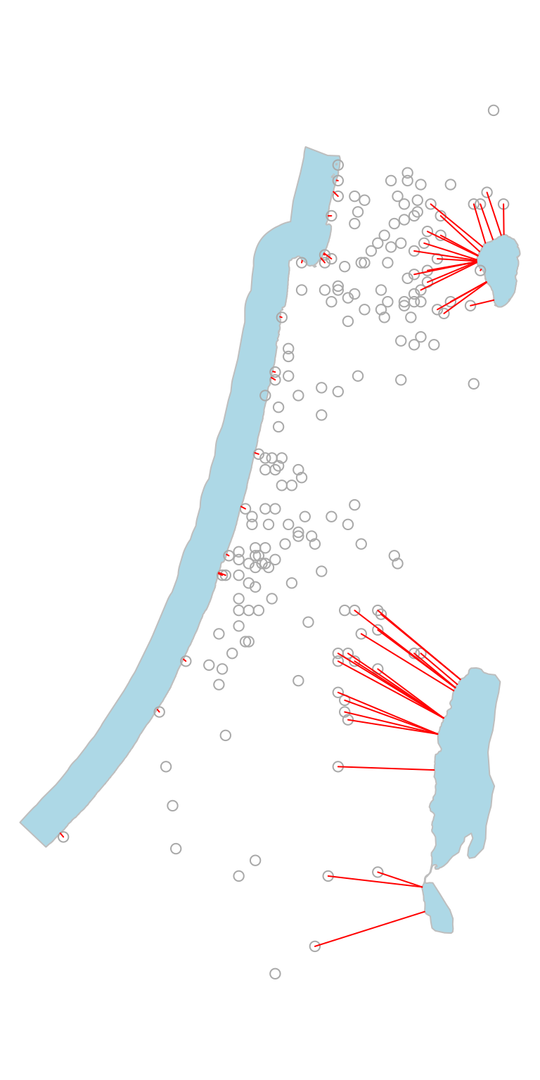

$Nearest 20 \texttt{towns} features from each \texttt{water} polygon$

Nearest 20 features from each polygon

Michael Dorman

2024-04-17

Introduction

Package purpose

Installation

Sample data

Usage examples

The `st_nn` function

The `st_connect` function

Dense matrix representation

k-Nearest neighbors where `k>0`

Distance to nearest neighbors

Search radius

Spatial join

Binding distances to join result

Polygons

Introduction to package nngeo

Michael Dorman

2024-04-17

Introduction

Package purpose

Installation

Sample data

Usage examples

The st_nn function

The st_connect function

Dense matrix representation

k-Nearest neighbors where k>0

Distance to nearest neighbors

Search radius

Spatial join

Binding distances to join result

Polygons

Introduction to package `nngeo`

The `st_nn` function

The `st_connect` function

k-Nearest neighbors where `k>0`