Introduction
The mapsapi package provides an interface to the Google
Maps APIs, currently four of them:
Functions mp_directions, mp_matrix and
mp_geocode are used to access the Directions, Matrix and
Geocode APIs, respectively. They return an xml_document
object (package xml2) with the response contents.
Given a directions response, functions
mp_get_routesandmp_get_segmentscan be used to process the response document into a spatial layer. Functionmp_get_routesgives each alternative as a separate line, while functionmp_get_segmentsgives each segment (that is, a portion of the route associated with specific driving instructions) as a separate line.Given a distance matrix response, function
mp_get_matrixcan be used to obtain distance/duration matrices.Given a geocode response, functions
mp_get_pointsandmp_get_boundscan be used to obtain geocoded locations as a point or polygon (bounds) layer.
The fourth function mp_map is used to access the Maps
Static API. It returns a stars raster RGB image, which can
be used as background in maps.
Installation
The CRAN version can be installed with:
install.packages("mapsapi")The development version can be installed using
remotes:
install.packages("remotes")
remotes::install_github("michaeldorman/mapsapi")
Once installed, the package can be loaded with
library:
A Google Maps APIs key is required to use the package:
key = "AIz....."Directions
The following expression queries the Directions API for driving
directions from Tel-Aviv and Haifa. Note that locations can be specified
as a coordinate pair, a textual address or an sf spatial
object. For example:
doc = mp_directions(
  origin = c(34.81127, 31.89277),
  destination = "Haifa",
  alternatives = TRUE,
  key = key,
  quiet = TRUE
)
Alternatively, we can use the sample response data included in the packages:
library(xml2)
doc = as_xml_document(response_directions_driving)
Given the response object, we can use mp_get_routes to
create a spatial layer of route lines:
r = mp_get_routes(doc)Here is the resulting object:
r## Simple feature collection with 2 features and 11 fields
## Geometry type: LINESTRING
## Dimension: XY
## Bounding box: xmin: 34.76391 ymin: 31.87341 xmax: 35.10642 ymax: 32.79439
## Geodetic CRS: WGS 84
## alternative_id leg_id summary distance_m distance_text
## 1-1 1 1 Yitzhak Rabin Hwy/Route 6 126121 126 km
## 2-1 2 1 Hwy 2/Kvish HaHof 122251 122 km
## duration_s duration_text duration_in_traffic_s duration_in_traffic_text
## 1-1 5265 1 hour 28 mins NA NA
## 2-1 5402 1 hour 30 mins NA NA
## departure_time arrival_time geometry
## 1-1 <NA> <NA> LINESTRING (34.81144 31.892...
## 2-1 <NA> <NA> LINESTRING (34.81144 31.892...and a visualization using leaflet:
library(leaflet)
pal = colorFactor(palette = "Dark2", domain = r$alternative_id)
leaflet() %>%
  addProviderTiles("CartoDB.DarkMatter") %>%
  addPolylines(data = r, opacity = 1, weight = 7, color = ~pal(alternative_id))
Separate segments can be extracted from the same response using
mp_get_segments:
seg = mp_get_segments(doc)Here are the first six features of the resulting object:
head(seg)## Simple feature collection with 6 features and 12 fields
## Geometry type: LINESTRING
## Dimension: XY
## Bounding box: xmin: 34.80859 ymin: 31.88656 xmax: 34.82317 ymax: 31.89256
## Geodetic CRS: WGS 84
## alternative_id leg_id segment_id summary travel_mode
## 1-1-1 1 1 1 Yitzhak Rabin Hwy/Route 6 driving
## 1-1-2 1 1 2 Yitzhak Rabin Hwy/Route 6 driving
## 1-1-3 1 1 3 Yitzhak Rabin Hwy/Route 6 driving
## 1-1-4 1 1 4 Yitzhak Rabin Hwy/Route 6 driving
## 1-1-5 1 1 5 Yitzhak Rabin Hwy/Route 6 driving
## 1-1-6 1 1 6 Yitzhak Rabin Hwy/Route 6 driving
## instructions
## 1-1-1 Head <b>southwest</b> on <b>Bnei Moshe St</b> toward <b>Negba St</b>
## 1-1-2 Turn <b>left</b> onto <b>Negba St</b>
## 1-1-3 Turn <b>left</b> onto <b>Rachel Hirshenzon St</b>
## 1-1-4 Turn <b>right</b> onto <b>Herzl St</b>/<wbr/><b>Route 412</b>
## 1-1-5 Turn <b>left</b> onto <b>Abarbanel St</b>
## 1-1-6 At the roundabout, continue straight onto <b>Derech Jerusalem</b>
## distance_m distance_text duration_s duration_text departure_time
## 1-1-1 322 0.3 km 65 1 min <NA>
## 1-1-2 180 0.2 km 36 1 min <NA>
## 1-1-3 327 0.3 km 75 1 min <NA>
## 1-1-4 548 0.5 km 108 2 mins <NA>
## 1-1-5 503 0.5 km 83 1 min <NA>
## 1-1-6 364 0.4 km 52 1 min <NA>
## arrival_time geometry
## 1-1-1 <NA> LINESTRING (34.81144 31.892...
## 1-1-2 <NA> LINESTRING (34.80859 31.890...
## 1-1-3 <NA> LINESTRING (34.80968 31.889...
## 1-1-4 <NA> LINESTRING (34.81257 31.891...
## 1-1-5 <NA> LINESTRING (34.81437 31.886...
## 1-1-6 <NA> LINESTRING (34.81956 31.887...and a visualization:
pal = colorFactor(
  palette = sample(colors(), length(unique(seg$segment_id))),
  domain = seg$segment_id
  )
leaflet(seg) %>%
  addProviderTiles("CartoDB.DarkMatter") %>%
  addPolylines(opacity = 1, weight = 7, color = ~pal(segment_id), popup = ~instructions)
Distance Matrix
The following expression queries the Distance Matrix API to obtain a matrix of driving distance and duration between all combinations of three locations: Tel-Aviv, Jerusalem and Beer-Sheva.
locations = c("Tel-Aviv", "Jerusalem", "Beer-Sheva")
doc = mp_matrix(
  origins = locations,
  destinations = locations,
  key = key,
  quiet = TRUE
)
Alternatively, we can use the sample response data included in the packages:
doc = as_xml_document(response_matrix)The mp_get_matrix function can then be used to process
the XML response into a matrix. Possible values of the
matrix include:
-
distance_m—Distance, in meters -
distance_text—Distance, textual description -
duration_s—Duration, in seconds -
duration_text—Duration, textual description
m = mp_get_matrix(doc, value = "distance_m")
colnames(m) = locations
rownames(m) = locations
m
## Tel-Aviv Jerusalem Beer-Sheva
## Tel-Aviv 0 66866 108728
## Jerusalem 68524 0 118083
## Beer-Sheva 110858 106562 0Geocode
The following expression queries the Directions API for geocoding a single address:
doc = mp_geocode(
  addresses = "Tel-Aviv",
  key = key,
  quiet = TRUE
)
Alternatively, we can use the sample response data included with the package:
doc = list("Tel-Aviv" = as_xml_document(response_geocode))Given the response object, we can use mp_get_points to
create a spatial layer of geocoded point locations:
pnt = mp_get_points(doc)
pnt
## Simple feature collection with 1 feature and 5 fields
## Geometry type: POINT
## Dimension: XY
## Bounding box: xmin: 34.78177 ymin: 32.0853 xmax: 34.78177 ymax: 32.0853
## Geodetic CRS: WGS 84
## id status address address_google location_type
## 1 1 OK Tel-Aviv Tel Aviv-Yafo, Israel APPROXIMATE
## pnt
## 1 POINT (34.78177 32.0853)Here is a visualization using leaflet:
leaflet() %>%
  addProviderTiles("CartoDB.DarkMatter") %>%
  addCircleMarkers(data = pnt)
Or the bounds:
bounds = mp_get_bounds(doc)
bounds
## Simple feature collection with 1 feature and 4 fields
## Geometry type: POLYGON
## Dimension: XY
## Bounding box: xmin: 34.74252 ymin: 32.02925 xmax: 34.85198 ymax: 32.14661
## Geodetic CRS: WGS 84
## id status address address_google geometry
## 1 1 OK Tel-Aviv Tel Aviv-Yafo, Israel POLYGON ((34.74252 32.02925...And a visualization using leaflet:
leaflet() %>%
  addProviderTiles("CartoDB.DarkMatter") %>%
  addPolygons(data = bounds)
Static maps
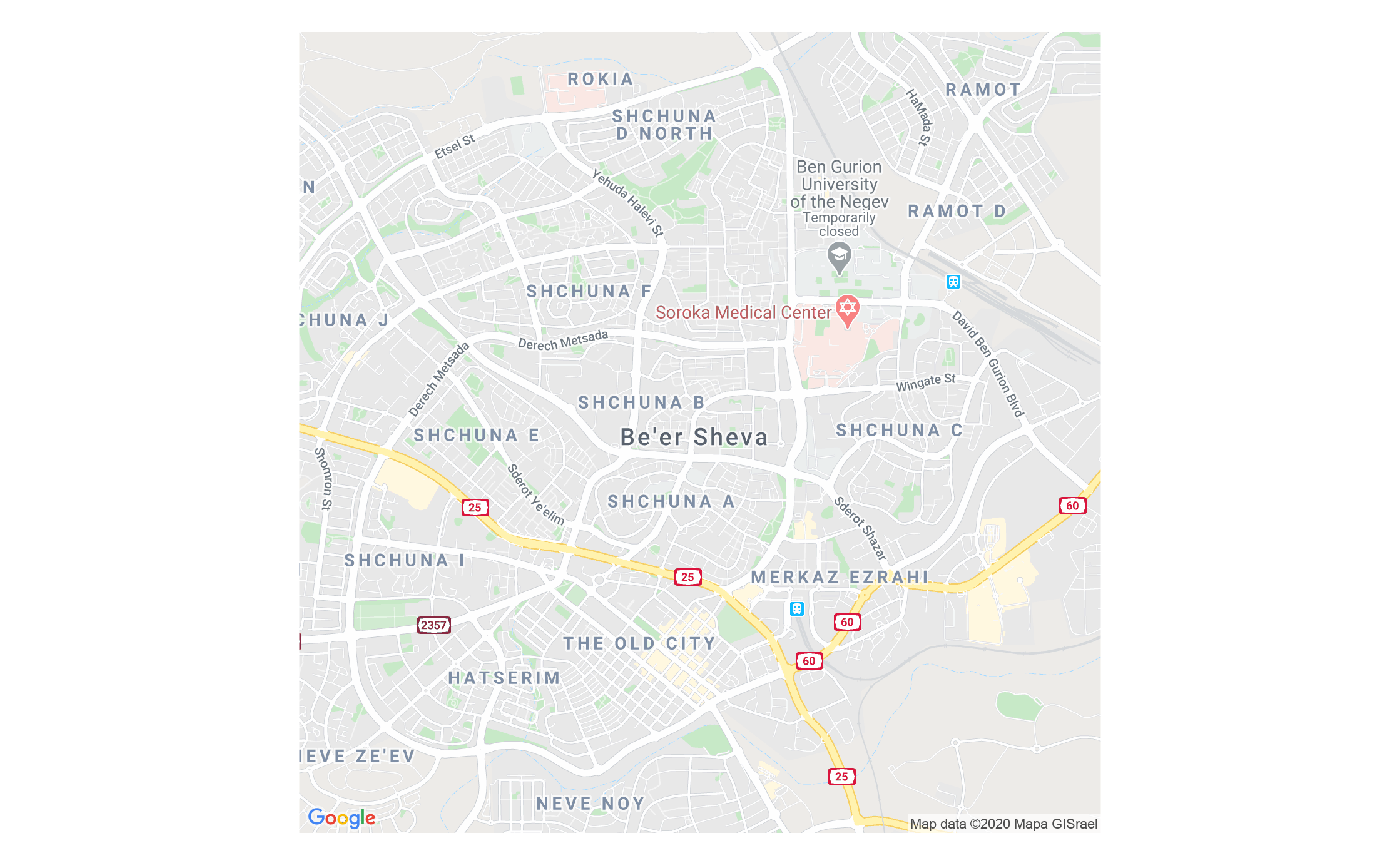
The mp_map function can be used to access the Maps
Static API to download an RGB image with a map.
Here is an example:
r = mp_map(center = "31.253205,34.791914", zoom = 14, key = key, quiet = TRUE)Alternatively, we can use the sample response data included with the package:
r = response_mapThe result is a stars raster, which can be plotted with
plot:
## Loading required package: abind## Loading required package: sf## Linking to GEOS 3.10.2, GDAL 3.4.1, PROJ 8.2.1; sf_use_s2() is TRUE
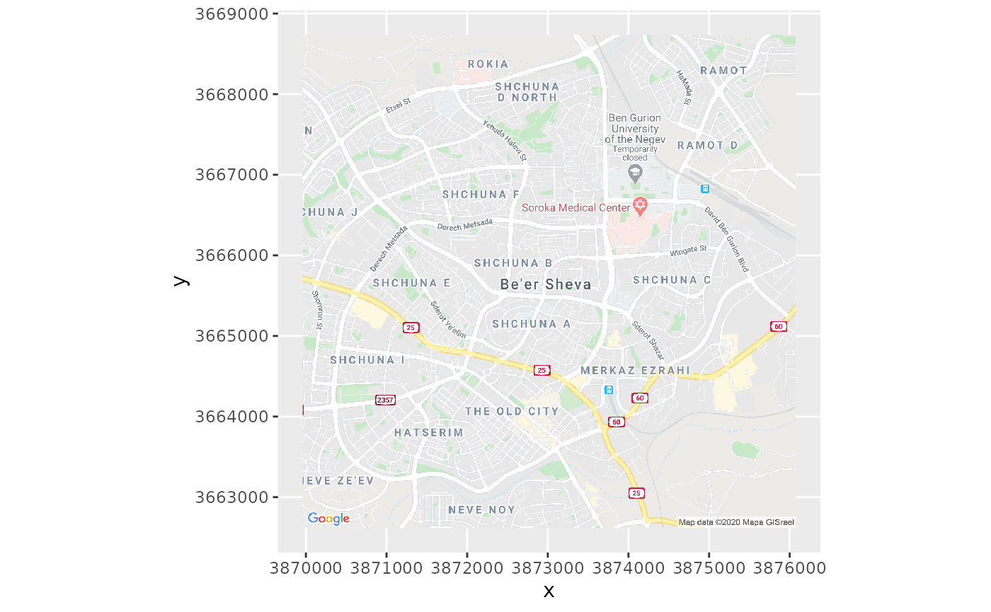
or with ggplot2:
library(ggplot2)
cols = attr(r[[1]], "colors")
ggplot() +
  geom_stars(data = r, aes(x = x, y = y, fill = color)) +
  scale_fill_manual(values = cols, guide = FALSE) +
  coord_sf()
## Warning: The `guide` argument in `scale_*()` cannot be `FALSE`. This was deprecated in
## ggplot2 3.3.4.
## ℹ Please use "none" instead.
## This warning is displayed once every 8 hours.
## Call `lifecycle::last_lifecycle_warnings()` to see where this warning was
## generated.