Spatial networks - First attempt

This document describes a preliminary workflow for familiarizing with using igraph to represent a spatial network. igraph is a package for network analysis, with the main data structure (igraph) used to represent a network. The term spatial network hereby refers to any network where both the vertices and the edges are associated with spatial features. For example, in a transportation network the vertices may correspond to junctions, bus stops, etc., while edges may correspond to the road segments connecting them.

In the following simple network, vertices correspond to US state centroids, while edges are straight line connections between the centroids. Not all possible vertex combinations are connected, however. We are going to connect only those centroids that correspond to states sharing a common boundary.

As a first step, let us obtain a SpatialPolygonsDataFrame object of US states -

library(rgdal)
library(rgeos)
library(igraph)

# Read states layer from a GeoJSON file
url = "https://raw.githubusercontent.com/alignedleft/d3-book/master/chapter_12/us-states.json"
state = readOGR(
  dsn = url, 
  layer = "OGRGeoJSON", 
  stringsAsFactors = FALSE, 
  verbose = FALSE
  )

# Transform to US-Atlas projection
state = spTransform(
  state, 
  "+proj=laea +lat_0=45 +lon_0=-100 +x_0=0 +y_0=0 +a=6370997 +b=6370997 +units=m +no_defs"
  )

# Assign state names to 'row.names'
row.names(state) = state$name

The attribute table of the state layer has the following structure. Note that we assigned state names to the row.names property. These are going to be the vertex names in the network.

head(state@data)

##            id       name
## Alabama    01    Alabama
## Alaska     02     Alaska
## Arizona    04    Arizona
## Arkansas   05   Arkansas
## California 06 California
## Colorado   08   Colorado

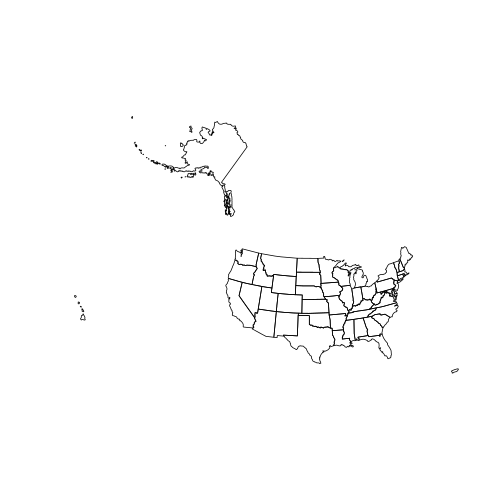
And here is a plot of the state layer:

plot(state)

One method to create an igraph object is to convert an adjacency matrix into igraph using function graph_from_adjacency_matrix. Since we would like to create edges only between those states that share a common boundary, our (52×52) matrix will have the value of 0 for all state×state combinations where there is no common boundary. Moreover, for those state pairs that do share a common boundary, we will give each edge a weight equal to the straight line distance between the centroids. That way, our network is going to be weighted, with weight representing an approximate distance among locations within the given states.

# Calculate 'SpatialPoints' layer of state centroids
ctr = gCentroid(state, byid = TRUE)

# Calculate pairwise logical matrix on feature intersection
m = gIntersects(state, byid = TRUE)

# Calculate pairwise distance matrix (in km)
d = gDistance(ctr, byid = TRUE) / 1000

# Assign 0 for 'no intersection', otherwise keep centroid distance
d[!m] = 0

Here are the first 5 rows and columns of the resulting matrix. Zero values mean that the states do not share a common border; non-zero values represent geographical distance (in km) between state centroids. For example, we can see that among the first five states only California and Arizona share a common boundary, and the distance between their centroids is 780 km.

d[1:5, 1:5]

##            Alabama Alaska  Arizona Arkansas California
## Alabama          0      0   0.0000        0     0.0000
## Alaska           0      0   0.0000        0     0.0000
## Arizona          0      0   0.0000        0   779.6966
## Arkansas         0      0   0.0000        0     0.0000
## California       0      0 779.6966        0     0.0000

Creating the igraph object goes as follows:

g = graph_from_adjacency_matrix(d, mode = "undirected", weighted = TRUE)

Thanks to the mode = "undirected" argument, the geographical distance is now stored in the weight property of each edge:

E(g)$weight[1:5]

## [1] 612.1047 318.3124 266.2254 345.7358 779.6966

Additionally, we can keep the x and y coordinates as vertex properties:

V(g)$x = coordinates(ctr)[, 1]
V(g)$y = coordinates(ctr)[, 2]

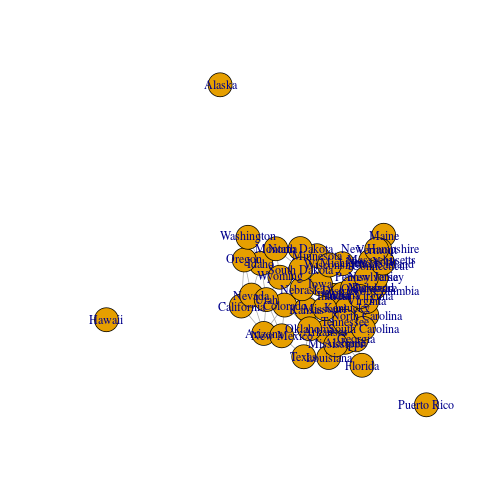
The network can be visualized with plot.igraph. Since vertices have x and y properties (which are spatial coordinates), their placement corresponds to spatial location:

plot(g)

This representation does not cover all spatial uses, however. We would also like to have the vertices and edges associated with features (points and lines, in this example). For example, when we employ network analysis methods such as shortest path or community detection we would like to get the corresponding spatial subsets, such as a line representing the path in space, or the a subset of vertices representing a community. How can we do this? A basic approach is outlined below.

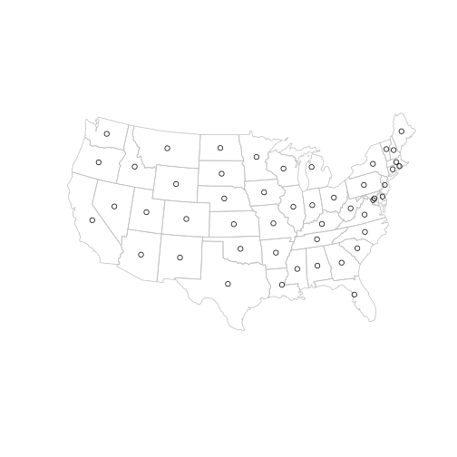
To represent the vertices we can simply use the centroid layer ctr created earlier. (only the contigous USA states are plotted below for clarity)

main = state[!state$name %in% c("Alaska", "Hawaii", "Puerto Rico"), ]
plot(main, border = "grey")
plot(ctr, add = TRUE, pch = 1)

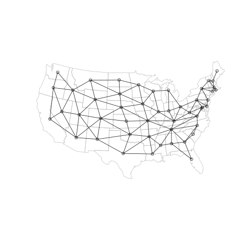
Creating the edge representation is a little more complicated. To do that, we need to make a line layer where each feature is a line (composed of two points) corresponding to a given vertex in our igraph object g.

The first step is to summarize edge name pairs for each vertex in g:

edges = get.edgelist(g)
edges = data.frame(
  v1 = edges[,1], 
  v2 = edges[,2], 
  stringsAsFactors = FALSE
  )
head(edges)

##        v1          v2
## 1 Alabama     Florida
## 2 Alabama     Georgia
## 3 Alabama Mississippi
## 4 Alabama   Tennessee
## 5 Arizona  California
## 6 Arizona    Colorado

For example, we see that the first two edges connect Alabama with Florida and with Georgia, respectively:

E(g)[1:2]

## + 2/109 edges (vertex names):
## [1] Alabama--Florida Alabama--Georgia

The second step is to make a SpatialLines object representing those edges. This can be done by sequentially connecting point-pairs from ctr with a for loop going over the rows in the edges table. Line construction itself is hereby performed with the shadow::ray function:

# Start with empty list
l = NULL 

for(i in 1:nrow(edges)) # For each edge
  l = c(
    l, 
    # Create 'SpatialLines' between the corresponding vertices
    shadow::ray( 
      ctr[edges$v1[i], ], 
      ctr[edges$v2[i], ]
      )
    )

# Combine all lines into one 'SpatialLines' object
l = do.call(rbind, l) 

Here is the result:

plot(main, border = "grey")
plot(ctr, add = TRUE, pch = 1)
plot(l, add = TRUE)

At this point we have:

• A network object g representing the relation between vertices (states).
• A SpatialPoints object ctr representing vertex locations (state centroids).
• A SpatialLines object l representing edge locations (straight lines between state centroids).

For now, the association between these three objects is based on the following:

• The order of ctr corresponds to the order of vertices in g.
• The order of l corresponds to the order of edges in g.

Thus, any statistical or descriptive calculation involving vertices and edges from g can later on be expressed using their spatial representation.

For example, we can find out the shortest path from Texas to Washington, in terms of vertex and edge IDs:

# Find shortest path
p = shortest_paths(g, "Texas", "Washington", output = "both")

# The 'vpath' component contains the vertex IDs on the path
p$vpath

## [[1]]
## + 5/52 vertices, named:
## [1] Texas      New Mexico Utah       Idaho      Washington

unlist(p$vpath)

##      Texas New Mexico       Utah      Idaho Washington 
##         44         32         45         13         48

# The 'epath' component contains the edge IDs on the path
p$epath

## [[1]]
## + 4/109 edges (vertex names):
## [1] New Mexico--Texas      New Mexico--Utah       Idaho     --Utah      
## [4] Idaho     --Washington

unlist(p$epath)

## [1] 93 94 39 40

The corresponding point and line layer can be created by subsetting the full layers:

p_vertices = unlist(p$vpath)
p_edges = unlist(p$epath)
p_ctr = ctr[p_vertices, ]
p_l = l[p_edges, ]

Let’s visualize the path’s vertices and edges in red, with the full network in the background:

plot(main, border = "grey")
plot(p_l, add = TRUE, col = "red", lwd = 3)
plot(p_ctr, add = TRUE, col = "red", pch = 16, cex = 1)
plot(l, add = TRUE)
plot(ctr, add = TRUE, pch = 1)

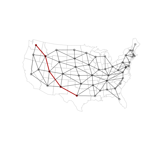
We can see that the first step in the path goes from Texas to New Mexico. What if these two states suddenly became ‘more distant’ from each other?

E(g)[from("Texas") & to("New Mexico")]$weight = 2000

The new path would then bypass New Mexico, going through Oklahoma instead:

p = shortest_paths(g, "Texas", "Washington", output = "both")
p$vpath

## [[1]]
## + 6/52 vertices, named:
## [1] Texas      Oklahoma   Colorado   Wyoming    Idaho      Washington

p$epath

## [[1]]
## + 5/109 edges (vertex names):
## [1] Oklahoma--Texas      Colorado--Oklahoma   Colorado--Wyoming   
## [4] Idaho   --Wyoming    Idaho   --Washington

p_vertices = p$vpath[[1]]
p_edges = p$epath[[1]]

And here is the new plot. The vertex we made more ‘distant’ is marked in yellow:

p_ctr = ctr[p_vertices, ]
p_l = l[p_edges, ]

plot(main, border = "grey")
plot(p_l, add = TRUE, col = "red", lwd = 3)

# Highlight the edge we made 'more distant'
plot( 
  l[E(g)[from("Texas") & to("New Mexico")], ], 
  add = TRUE, 
  col = "yellow", 
  lwd = 3
  )

plot(p_ctr, add = TRUE, col = "red", pch = 16, cex = 1)
plot(l, add = TRUE)
plot(ctr, add = TRUE, pch = 1)

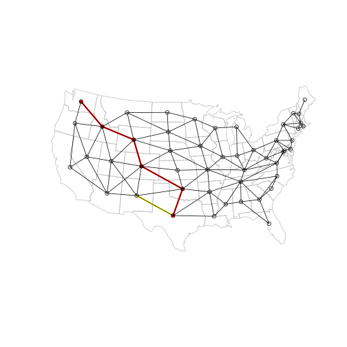
That’s it for now, thanks for reading!